If you’re familiar with what we do here in the Entertainment Engineering group at the University of Derby, you’ll know that we like to create useful bits of software and make them free for anyone to try out.
Just this week saw the release of the Low-Frequency Acoustics Toolbox (LowFAT), which is an updated and streamlined version of the FDTD Simulation Toolbox, which was originally developed back in 2008.
LowFAT allows you to run acoustic simulations in rectangular or non-rectangular spaces (2D or 3D) with sound sources and measurement points placed wherever you like. Once the simulation is finished you can analysis the data in many different ways, including creating animations to visualize the sound propagation in the space.
While the full set of features is described in detail in the LowFAT User’s Guide, I thought it’d be useful to walk through a quick demo of the software.
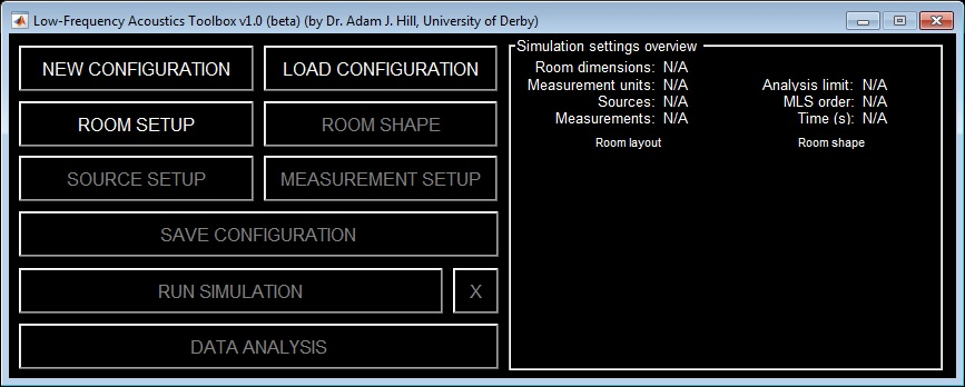
Let’s start by launching the application and selecting new configuration. You should see a window like this:
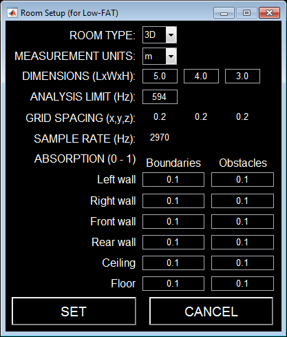
Then we’ll go into the room setup and define the space as shown:
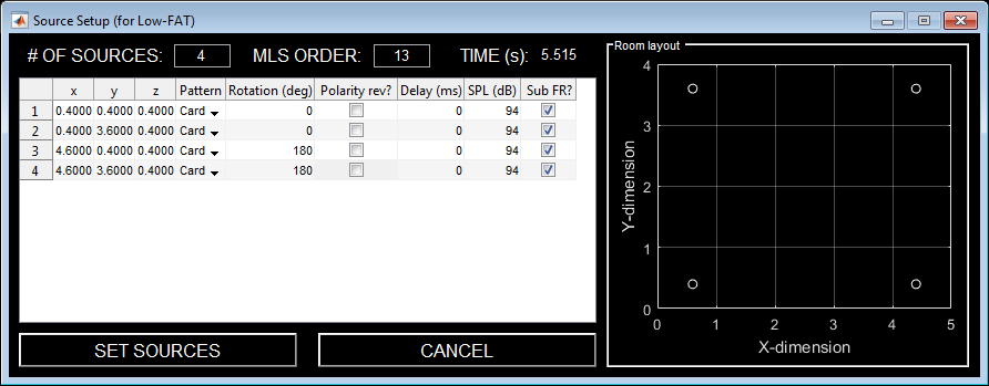
Now let’s say we want to have four subwoofers in the space, all with a cardioid polar pattern and facing into the room (along the x-axis) and placed in the room corners (40 cm from any surfaces).
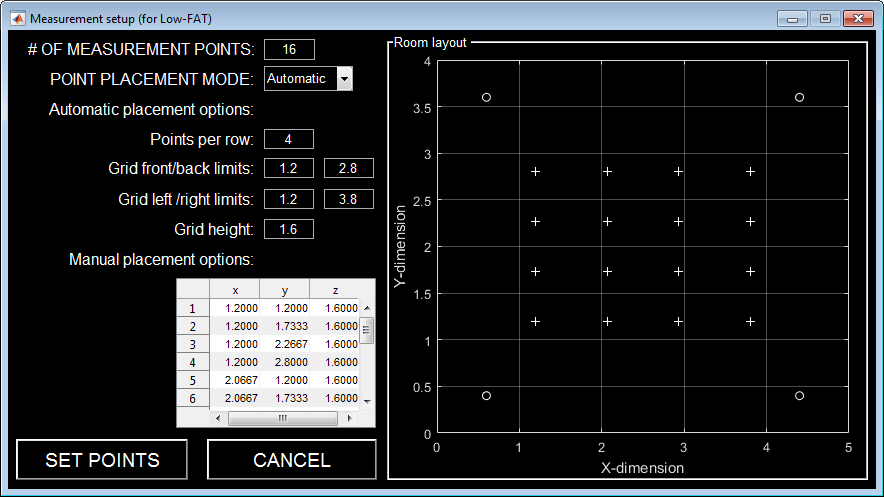
Lastly, we’ll create a 4 x 4 grid of measurement points with a height of 1.6 m.
Now it’s time to run the simulation. I’ll choose to save the full grid data so we can make animations later.
Now we’re ready to analyse the data!
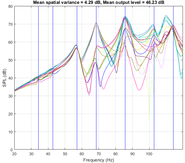
We’ll start with looking at the raw impulse responses. Looking at the magnitude responses (from 20 – 100 Hz) with the theoretical axial and tangential modes overlaid let’s us know if the simulation is reasonably accurate:
You can see that the four subs in the room corners (on the floor) prevents the lowest two axial modes form exciting, thus reducing the seat-to-seat variance in the magnitude response. The theoretical modes seem to line up nicely with the simulation, so it seems pretty accurate so far!
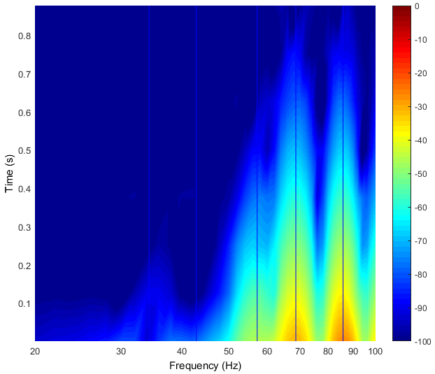
Bringing in the time domain, we can look at the spectrogram for point (2,2) in the measurement point grid.
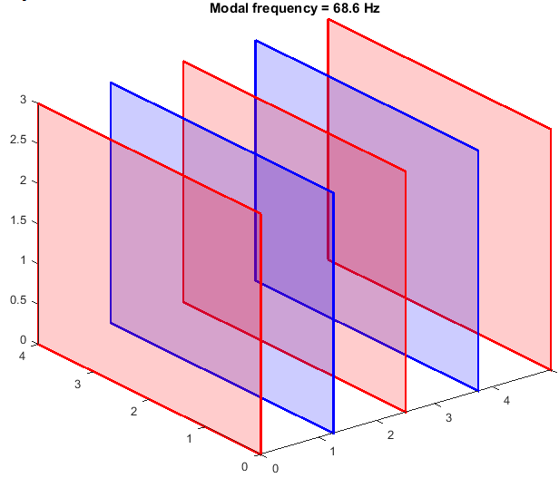
Let’s now look at the first horizontal axial mode (2, 0, 0) at 68.6 Hz and see what it’s doing in the room. I’ll change the source type to sinusoid and set the frequency. Then let’s look at the expected modal distribution.
Now, we can generate an animation to see if this is what we get. We’ll start with a 2D animation looking at a height of 1.6 m in the room.

Which we can also look at in 3D:

Finally, let say we want to hear how the low-frequency response differs from location to location. Tone bursts are great signals for this. Here’s a raw tone burst at 68.6 Hz compared to three of the measurement points: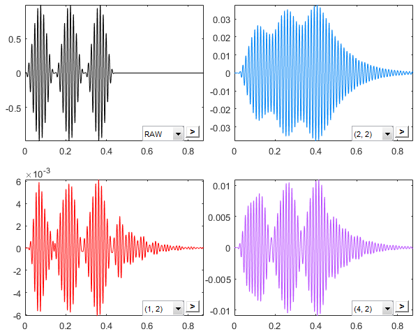
Clearly, the time (and magnitude) response of the tone bursts is very position-dependent. Let’s have a listen:
Raw:
(2,2):
(1,2):
(4,2):
Finally, we can load in an audio file and listen to how the low-frequency sounds (with the HF unaltered) at various locations:
(1, 1):
(1, 2):
(2, 1):
(2, 2):
If you were only running one subwoofer, then these differences would be even greater! We’ll save that for another post…
There’s much more you can do with the toolbox, but hopefully this gives you a feel for what’s possible. It’s currently a beta release, so try it out and please report back with any bugs you find.
Happy simulating!

